Propagation of Malware: Examining the Conficker Worm and SI, SIS, and SIR Models through Graphical Network Simulator-3

In this research paper, we addressed the propagation of malware through the Internet using concepts from graph theory and other aspects of network science. We focused on malware as downloaded attachments that have to be present on a physical device to have a real, detrimental impact on the host software. Throughout this study, we used a topographic model of a computer network as a base to test the efficacy of multiple propagation models. The reason for implementing and applying such simulations to the propagation of malware is due to the ongoing harmful effects of the proliferation of modern malware on computers.  This research expands on existing knowledge in this field by allowing users to predict potential implications and damage outputs of future attacks in advance so that users may be prepared for such threats. We used the Conficker worm as an example in order to study the damage that a piece of propagating malware does to a computer network. In order to do so, we analyzed the data from models, such as the SI, SIS, and SIR models, to study the virus propagation. We also provided more updated models of virus proliferation and compared them extensively. Because of the detrimental impacts of such cyber-attacks, it is crucial to examine ways to possibly mitigate the proliferation of malware through computers. Thus, the results of this paper  illustrates possible methods to mitigate the propagation of viruses or worms.

I. INTRODUCTION

Malware (portmanteau of the words “malicious” and “software”) is a category of programs that perform a detrimental action to a computer when initiated in the network. Common types of such malware include worms, viruses (autonomous replication), and Trojan horses (malware attached to seemingly inconspicuous files or programs). This research paper examines how computer malware, specifically worms, propagate from device-to-device as well as the consequences of such infections. While viruses require an active or already-infected host file in order to replicate, worms are stand-alone programs that attack other networks after self-replicating. In our study, we did not include viruses transmitted through websites that require downloads. By studying malware in the earlier stages of propagation, it will allow organizations to inhibit malware from infecting other devices and posing a significant threat. Using the Susceptible-Infected (SI), Susceptible-Infectious-Susceptible (SIS), and Susceptible-Infectious-Recovered (SIR) models outlined in previous studies, our research will allow data scientists to accurately predict how a virus or worm would propagate.

Ever since the mid-1900s when the first virus was introduced into a digital network, computer malware has been a significant threat to the technology sector. Every year, millions of people around the world are affected by computer viruses. The dangers of computer malware are particularly evident in instances where criminals have access to a person's personal information including, but not limited to, social security numbers, credit card information, addresses, and birth dates. Due to such dangerous threats, it is crucial to study computer malware in order to determine how to contain or even stop possible infections.

This research paper  mainly discusses the models in terms of the crypto-worm, “Conficker,” which was unleashed in 2008 after being created by Ukrainian programmers. Reported to have infected 11 million devices to date, Conficker is considered one of the most destructive worms ever unleashed. The Conficker worm is “headless,” as it is able to operate without a connection to the central server. As a result, the Conficker worm is one of the most long-reaching pieces of malware. The effects are also still visible past the initial infection date;A report released by the IT security company Trend Micro shows that about 15,000 machines were still infected by September 2017 [2]. Thus, the Conficker worm served as a precursor to several modern effective worms. The goal of this research paper is to study such pieces of malware in order to determine how to best contain these destructive threats.

This study includes multiple models from previous works. These models were utilized to define the features of various models pertaining to the propagation of the virus in a network. An additional simulation will also be used in order to model a network for testing, which will be derived from the software Graphical Network Simulator-3 (GNS3) [3].The model of the propagation is used to determine the pattern of which nodes, or the computers in the network, become infected the fastest, and subsequently how to stop the hypothetical infection at the optimal point. It can also be used to determine the average amount of time until the system reaches equilibrium or the point in time when the variables in the model become constant.

II. BACKGROUND AND LITERATURE REVIEW

Existing Models Utilized

Previous scholarship by Lajamonovich and Yorke (2002) proposed an SIS model over a network of n-dimensions [5]. This model established the existence of the endemic state. The endemic state is a non-zero value at which the infected population is maintained without the influence of external factors. This model is referred to when an SIS model is mentioned because the infected population moves back into a susceptible state after recovery, meaning that they can still catch the contagious agent.

Yang et al. (2012) included an SIR model [13]. This model was included due to the latency between the arrival of the virus to a host and the virus becoming active. Another central assumption is made upon the difference in time between the complete infection of a host and the host becoming infectious. The study also defined a virus equilibrium, which is based upon the time delays mentioned. Furthermore, the study corroborated that the virus equilibrium might become a Hopf Bifucrum, which signals a change in stability.

Serazzi and Zanero (2004) proposed a different model. Based on research data studying the Code Red v2 worm, the model used the probability of a worm randomly attacking a computer on the same network or another computer external to the network of the worm's host [9]. With the inclusion of bandwidth and propagation-based limitations, Serazzi and Zanero developed an equation similar to the infinite Random Constant Spread (RCS) model developed by Stanford, Paxson, and Weaver [10].

Zhang and Song (2017) investigated a model similar to the SIR model, but included four separate states instead of three. They added a state where an infected individual is barred from infecting others, such as situations of system failure or shutdown [14]. Certain delays, such as bifurcation parameters, led to changes in the virial equilibrium, which differed based on the critical value of the system. The volatility of the system changed as a result.

Related Works

In addition to using the methods described in the aforementioned  papers, a comparison was done between these papers regarding their procedures and their subsequent results in a study by Wenjun Mei et al. In this research paper, it discussed the spread of an arbitrary infectious disease over an arbitrary network and modeled it over a digital network. It also referred to the SI, SIS, and the SIR models, which is essential to interests concerning the propagation model of the computer malware. Furthermore, Serazzi and Zanero’s research  studied the optimization of propagation models to help predict possible computer malware threats and potential containment methods. In both of these papers, they explored computer modeling in networks, which would serve as a basis for this research in regard to the propagation of malware in computer networks. Models can include many factors, such as the limits of bandwidth,implications of delays,a graded infection model, and the effects of human intervention in propagation [14]. The models used include those developed in some of the following studies: Lajamonovich and Yorke 1976, Serrazi and Zanero 2004, Zhang and Song 2017, and Yang et al. 2012.

III. METHODS AND MATERIALS

Graphical Network Simulator-3 (GNS3) Simulation

In order to simulate the propagation of such infections over computer networks, the modeling program GNS3 was used. The malware and virus propagation is represented through the use of the software, which can model physical computer networks. The software was used in order to model how computer malware propagates between different devices, including how it might use an already infected host file to infect other programs (viruses) or whether it is a stand-alone (worms). Furthermore, this model is used to analyze the theoretical average time the virus takes to reach the endemic state, which is when the proportion of the infected population no longer changes.

SI, SIR, and SIS Models

In addition to using the GNS3 simulation, the SI, SIR, and SIS methodology was also used in order to create models that simulate the propagation of the worm. For the purpose of this study, the three models, first proposed by Kermak and McKendrick in 1927, can be used to model the spread of any type of contagious agent. In general, these models map the number of users that are susceptible, infected, or recovered. The susceptible population are those that are at risk of becoming infected, which is initially close to 100% of the population. For the infected population, it takes just a single infected node to spread the contagious agent. In the case of the SIR model only, the recovered population are those that become fully immune. FIG. 1 shows a basic diagram that depicts how each model works.

FIG. 1. A graphic representation of the SI, SIR and SIS models respectively.

Because the infected population cannot be treated in the SI model, the susceptible population continues to drop as the infected population increases. In the graph of an SI model, the susceptible population hits the endemic state where the variables remain constant. In the SIS model, the infected nodes can "recover" after getting infected but return back to the susceptible phase at the recovery rate. In the SIR model, the infected nodes transition into a state in which the given node is now completely immune.

SI Model Formula: x'(t)=s(t)x(t)

SIS Model Formula: x'(t)=s(t)x(t)-x(t)

SIR Model Formulas: s'(t)=-s(t)x(t)

x'(t)=s(t)x(t)-x(t)

r'(t)=x(t)

In the above equations, 𝛃 represents the infection rate, while 𝛄 represents the recovery rate. In the SIR model, the infected nodes will be cured if 𝛄 > 𝛃. In the formulas, x(t) is the infected population, s(t) is the susceptible population, and r(t) is the recovered population at time t. Analyzing these models help us determine how computer malware infects other devices.

The Serazzi and Zanero Model

Serazzi and Zanero proposed an entirely new model based on research data on the Code Red v2 and Slammer worms in conjunction with an SIS model [9]. The model used the rate of incoming and outgoing worm-based traffic reduced by the limitations of bandwidth as a function of s(t) or the susceptible population. FIG. 2 shows the equation that is based on the Serazzi-Zanero model. Furthermore, the expression (T - Ti) represents the idea that an infected host can become infectious after a delay.

FIG. 2. Model developed by Serazzi and Zanero

Other Crucial Models

In addition, the methods described in various past research papers were also used to make a comparison between procedures and their subsequent results, including: “Opinion Dynamics and the Evolution of Social Power in Influence Networks” [4], “On the Dynamics of Deterministic Epidemic Propagation over Networks” [6], and “Computer Virus Propagation Models” [9], which were discussed in the Background and Literature Review section.

IV. DATA AND RESULTS

Modeling the Infection of the Conficker Worm

The data used originated from the University of California, San Diego's Network Telescope, managed by the Center for Applied Internet Data Analysis (CAIDA) [11]. The data pertained to the spread of the Conficker worm through machines from November 20 and 21 in 2008. Specifically, the Network Telescope captured network data on the number of devices infected by the malware within a 24-hour period from the two days mentioned. Through these means, a graph of the data was produced by CAIDA by mapping the number of devices infected to specific time-stamps throughout the 24-hour period. Furthermore, the nodes on the graph of FIG. 3 were plotted through 1-hour increments, and at its peak, 114,911 unique IP addresses were infected by the worm [1].

FIG. 3. A graph representing the population of computers infected through the Conficker worm

SI, SIS, and SIR Graphs

In addition to plotting the nodes of the infected population, SI, SIS, and SIR graphs were also created to represent the infected rate and recovery rate after the worm is introduced into the computer network. The SI model was used because it depicts how long it takes for a worm to propagate through a digital network without a recovery rate. The model used in FIG. 4 implies that in the absence of recovery, a threatening worm can infect a large population of computers in just a day.

In FIG. 5, a modified SIS version of the Serazzi-Zanero graph was used to determine how quickly computers can “recover” back into the susceptible state at the recovery rate, 𝛄. In the graph, the anomaly in the infection rate represents the drop in the number of infected computers. One of the limitations that was found while working with the modified Serazzi-Zanero model was the fact that the two subpopulations did not add up to the total number of computers after reaching equilibrium. Although the issue could not be fixed due to the time constraints, the plotted data prior to equilibrium showed us how quickly some computers can still reach the susceptible state after infection. In the long run, the result is beneficial because more computers will recover at a quicker rate.

FIG. 4. Potential Propagation of Conficker: SI Model

In FIG. 5, a modified SIS version of the Serazzi-Zanero graph was used to determine how quickly computers can “recover” back into the susceptible state at the recovery rate, 𝛄. In the graph, the anomaly in the infection rate represents the drop in the number of infected computers. One of the limitations that was found while working with the modified Serazzi-Zanero model was the fact that the two subpopulations did not add up to the total number of computers after reaching equilibrium. Although the issue could not be fixed due to the time constraints, the plotted data prior to equilibrium showed us how quickly some computers can still reach the susceptible state after infection. In the long run, the result is beneficial because more computers will recover at a quicker rate.

FIG. 5. Potential Propagation of Conficker: Modified Serazzi-Zanero SIS Model

The SIR model was used to demonstrate how quickly these computers can recover after being infected. In FIG. 6, the gradual increase of recovered computers after a decline in the susceptible and infection populations is good because it implies that fewer computers will be damaged in the long run. The initial spike in the infected population depicts the high infection rate of malware.

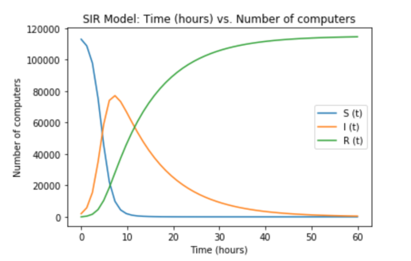
FIG. 6. Potential Propagation of Conficker: SIR Model

The Test Network

Worms, such as the Conficker, can debilitate the larger networks of considerable organizations (e.g. power grids, large companies, and government and military branches). However, the risk to smaller organizations, such as hospitals and small business, is even higher due to the weak security measures of the Internet of Things (IOT) [12]. To analyze this risk, GNS3 was used to build a topographical model of a test network.

FIG. 7. The test network created on GNS3

The network in FIG. 7 shows a simple star network, which is a common industry deployment. The icons labeled 'R1' through 'R5' signify virtual Cisco c3725 routers. The 'VPCS 1-16' are virtual placeholders which are connected by Fast Ethernet (100 mbps) to the virtual router.

FIG. 8. The SI Model over the Test Network

The graph in FIG. 8 represents an SI-based model graphed from the GNS3 test network. The graph shows the total number of iterations, or the number of times that the code was run, and the total number of nodes, including computers and routers. This graph depicts a theoretical simulation of the propagation of an arbitrary malware over the tested network with 16 computers and 5 routers. 

Theoretical Average Equilibrium Time

The time of equilibrium is the point in time at which all variables in a system remain constant and have no rate or a negligible rate of change. The Average Equilibrium Time can be found through the three equations defined below, which establish the basis for “equilibrium” in the models. In the formulas, N represents the total population and s(t) and x(t) represent the susceptible and infected populations respectively as functions of time t. In the SIR model, r(t) represents the recovered population.

s(t)+x(t)+r(t)=N

s(t+1)s(t)

x(t+1)x(t)

r(t+1)r(t)

If a value of t can be found where a model reaches equilibrium, and the sum of t represents the times of equilibrium across multiple models of the same network, the Average Equilibrium Time, a(n), can be found through a(n)= k=1ntkn.

The Average Equilibrium Time serves as an important value in the analysis of propagation models, as it represents the time at which the most damage has been done. The individual time values of equilibrium can vary due to many factors of the model. By taking the average of the set of individual equilibrium time values, the Average Equilibrium Time should more closely fit the actual spread of infection. Applied to the modified Serazzi-Zanero SIS model, the theoretical average equilibrium time clocks in at about 21 hours, signaling that the maximum number of computers will theoretically be infected by that time. Similarly, the calculation for the SI model signals equilibrium after 53 hours. In addition, the value for the SIR model is at approximately 59 hours. Based on the SI, SIS, and SIR models of the same network–which can all be applied in different scenarios–, the Average Equilibrium Time is approximately 44.33 hours.

Ⅴ. DISCUSSION

After reviewing the various propagation models, we suggest an approach to determining the optimal point in a network before the prevention of the spread of malware. As Conficker, a worm which can transmit itself without human intervention, is one of the fastest spreading worms because of its nature, it is necessary to have a proper prevention strategy to deter this threat as well as future ones. This is in contrast to other worms like Wanna-Cry,a ransomware crypto-worm used in a global attack in 2017, which sometimes have kill switches and other vulnerabilities that can lead to the end of an outbreak. Previously, in order to prevent such malware from spreading to other machines, the default solution was to use a reactive measure, which for most organizations is to disconnect the computer, reformat, and reconnect the computer back to the network. However, the crude nature of this resolution is demonstrated in Serazzi and Zanero’s research paper. Thus, more proactive solutions must be used. Organizations can take advantage of a vast number of software, firmware, and physical tools to protect their networks. A simple but ignored preventive measure is the installation of updates. Another measure can be the use of a firewall or any anti-virus software to detect the signatures of certain types of malware.

Even with the best malware defenses, networks can become susceptible to infiltration and can suffer from the fallout of a cyberattack. Thus, an agenda of prevention must aim to contain the malware in order to reduce the amount of damage from an attack. An important countermeasure can be the mass deployment of security updates and software. This is pertinent to the nodes of a network that have a high centrality or high concentration of connections. This is because making these nodes resistant or even immune to infection also protects the nodes directly connected to this central node. However, in the case of a growing infection in a vulnerable network, the best option would be to contain the infection before the largest rate of increase, which is considered in respect to the growth of the infected population in the case of the SI, SIS, and SIR models. With the combination of determining the node in the network with the highest degree centrality and subsequently blocking the connection between the central and surrounding nodes, as well as stopping the spread before the predicted peak infection rate, this method serves as the optimal method to stopping the propagation of a given malware.

Ⅵ. CONCLUSION

Using the GNS3 simulation, it was determined that there are specific places where infections can be stopped before it can spread to various other devices. In addition, a CAIDA dataset was analyzed in order to apply similar models to the test network over the GNS3 software. However, the models used in this study are slowly becoming less and less predictive as malware continues to evolve. Because malware and cybersecurity are in a constant virtual arms race, it limits research to simulations and studies on past ransomware attacks. In order to ensure protection from malware threats, organizations must improve their methods of malware propagation prevention, including anti-virus software and recent security updates, on digital devices. The GNS3 simulation could be improved if the simulation was able to fully simulate the digital network by introducing an actual worm into the system. Likewise, the SI and SIR models could be improved upon by determining a more efficient mathematical way of computing the Average Equilibrium Time within the system.

In this study, we discussed various propagation models of malware based on the Conficker worm. We graphed the results and analyzed the properties of each graph, including the speed of the spread, time until the endemic point, as well as when the graph would reach its peak in terms of infection. We also compared each method to its subsequent graph and studied the features of it in order to determine possible ways to prevent infection at the most ideal point. In addition, we also used GNS3 to build a topographical model in which the multiple propagation models can be applied. We used this topographical model to show the possible ways the malware can spread to various hosts and how to contain it from the further infection of devices. Due to the fact that malware is evolving at an uneven rate, it becomes even harder to predict exactly what will be coming in the near future. As malware becomes more advanced, it becomes a crucial necessity that we develop modernized methods and tools as a safety precaution.

[1] Center for Applied Internet Data Analysis. UCSD Network Telescope – Code-Red Worms Dataset.2001. URL: http://www.caida.org/data/passive/codered_worms_dataset.xml.

[2] CONFICKER/DOWNAD 9 Years After: Examining its Impact on Legacy Systems.Dec. 2017. URL: https://blog.trendmicro.com/trendlabs-security-intelligence/conficker-downad-9-years-examining-impact-legacy-systems/.

[3] Jeremy Grossmann, Dominik Ziajka, and Piotr Pękala. Graphical Network Simulator-3. URL: www.gns3.org.
[4] Peng Jia et al. Opinion dynamics and the evolution of social power in influence networks. 2015.
[5] Lajamonovich and J A Yorke. A deterministic model for gonorrhea in a nonhomogeneous population.Nov. 2002. URL: https://www.sciencedirect.com/science/article/pii/0025556476901255.

[6] Wenjun Mei et al. “On the dynamics of deterministic epidemic propagation over networks”. In: Annual Reviews in Control44 (2017), pp. 116–128. DOI: 10.1016/j.arcontrol.2017.09.002.

[8] Steve Morgan. Global Ransomware Damage Costs Predicted To Exceed $8 Billion In 2018. Oct. 2018. URL: https://cybersecurityventures.com/global-ransomware-damage-costs-predicted-to-exceed-8-billion-in-2018/.

[9] Giuseppe Serazzi and Stefano Zanero. “Computer Virus Propagation Models”. In: Performance Tools and Applications to Networked Systems Lecture Notes in Computer Science(2004), pp. 26–50. DOI: 10.1007/978-3-540-24663-3_2.

[10] Stuart Staniford and Vern Paxson. “How to Own the Internet in Your Spare Time”. In: Proceedings of the 11th USENIX Security Symposium (Aug. 2002). URL: https://www.usenix.org/legacy/event/sec02/full_papers/staniford/staniford.pdf.

[11] The CAIDA UCSD Two Days in November 2008-July 2019. URL: https://www.caida.org/data/passive/telescope-2days-2008_dataset.xml.

[12] The odd, 8-year legacy of the Conficker worm”. In: WeLiveSecurity(Nov. 2016). URL: https://www.welivesecurity.com/2016/11/21/odd-8-year-legacy-conficker-worm/.

[13] Lu-Xing Yang et al. “A novel computer virus propagation model and its dynamics”. In: International Journal of Computer Mathematics89.17 (2012), pp. 2307–2314. DOI: 10.1080/00207160.2012.715388.

[14] Zizhen Zhang and Limin Song. “Dynamics of a Computer Virus Propagation Model with Delays and Graded Infection Rate”. In: Advances in Mathematical Physics 2017 (Jan. 2017), pp. 1–13. DOI: 10.1155/2017/4514935. URL: https://www.hindawi.com/journals/amp/2017/4514935/.